Basic Concepts of Statistics, Probability and Python

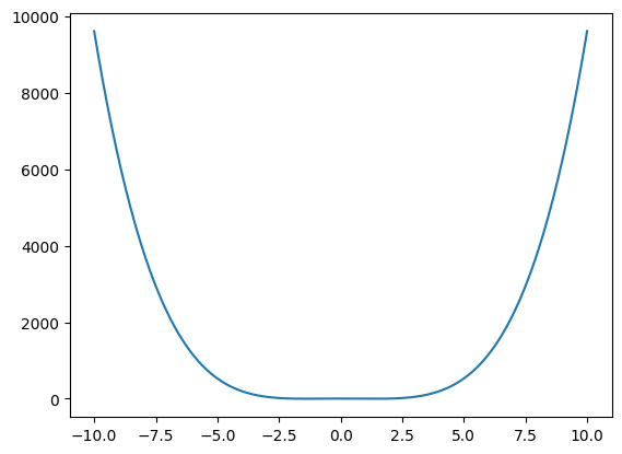
Create a Jupyter notebook and solve each exercise in an individual cell.

Each team must submit the Jupyter notebook and defend it on February 6, 2025. The defense will be carried out by one of the team members chosen at random.

Exercise 1: Mean and Median

Write a Python program that calculates the mean and median of a list of numbers.

Exercise 2: Standard Deviation

Write a Python program that calculates the standard deviation of a list of numbers.

Exercise 3: Data Visualization

Write a Python program that uses the matplotlib library to visualize a histogram of a list of numbers.

Exercise 4: Probability Distribution

Write a Python program that calculates the probability of an event occurring given a probability distribution (e.g. normal, binomial).

Exercise 5: Conditional Probability

Write a Python program that calculates the conditional probability of an event occurring given another event.

Exercise 6: Bayes’ Theorem

Write a Python program that applies Bayes’ theorem to update the probability of a hypothesis given new evidence.

Exercise 7: Correlation Coefficient

Write a Python program that calculates the correlation coefficient between two lists of numbers.

Exercise 8: Regression Analysis

Write a Python program that performs a simple linear regression analysis on a dataset.

Exercise 9: Random Number Generation

Write a Python program that generates random numbers from a specified probability distribution (e.g. normal, uniform).

Exercise 10:Function visualization - I

Generate a python code that allows the visualization (in one figure) of the real (blue) part and the imaginary (red) part, magnitude (green) and phase of the following signals: \[f\left(t\right) = e^{-j10 \pi t}\] \[g\left(t\right) = 10cos\left(2 \pi t\right) + j10sin\left(2 \pi t\right)\]

The visualization must be in the range of t \(\left[-10, 10\right]\)

Exercise 11: Function visualizartion - II

Generate a python code to show the following step function:

$$f(t) = \[\begin{cases} -t & \text{if } -5 \leq t \leq 0, \\ t & \text{if } 0 \leq t \leq 5, \\ 0 & Otherwise \end{cases}\]

$$

The visualization must be in the range of t \(\left[-10, 10\right]\)

Exercise 12: Physionet database

Download a record from the Physionet database EEG Signals from an RSVP Task (itrsvp) and create a script that enables the visualization of all the signals contained in the record. Make sure to use the correct amplitude and time units.

Data Creation

import numpy as np
import matplotlib.pyplot as plt

def h(x):
    return x**4 - 4*x**2 + 4

t = np.linspace(-10, 10, 1000)
h_t = h(t)

plt.plot(t,h_t)

[<matplotlib.lines.Line2D at 0x7f3ea7da36b0>]

Exercise 13: Numerical Diferentation

Determine the numerical derivative of the function h, represented as \(\left(\frac{dh}{dt}\right)\), via finite difference approximation. Subsequently, contrast this result with the numerical evaluation of the symbolic derivative, derived through analytical differentiation, to assess the precision of the numerical approach

Exercise 14: Numerical Integration

Determine the numerical integration of the function f, represented as \(\left(\int_{-10}^{10}{h(t)dt}\right)\), via trapezoidal rule. Subsequently, contrast this result with the numerical evaluation of the symbolic integral, derived through analytical differentiation, to assess the precision of the numerical approach

Exercise 15: Numerical solutions of ordinary differential equations (ODEs)

Solve the ODE \(\frac{dy}{dx} = 2x - 3y\) with initial condition y(0) = 1 using Euler’s Method. With a step 0f 0.1. Suppose that: \(x \in \left[0, 10\right]\) and \(y \in \left[1, 10\right]\)

Exercise 16: Numerical optimization

Minimize the function f(x) = x^4 - 4x^2 + 4 using Gradient Descent.